Visualization using the Matplotlib
Building the visualizer
The overall plan here is to derive a class that we will call MplPendulumVisualizer
from MplVisualizer. In its constructor,
we will lay down all the elements we want to use to visualize the system.
In our case these will be the beam on which the cart is moving, the cart and
of course the pendulum. Later on, the method
pymoskito.MplVisualizer.update_scene()
will be called repeatedly from the GUI to update the visualization.
We will start off with the following code:
 1# -*- coding: utf-8 -*-
 2import numpy as np
 3import pymoskito as pm
 4
 5import matplotlib as mpl
 6import matplotlib.patches
 7import matplotlib.transforms
 8
 9
10class MplPendulumVisualizer(pm.MplVisualizer):
11
12    # parameters
13    x_min_plot = -.85
14    x_max_plot = .85
15    y_min_plot = -.6
16    y_max_plot = .6
17
18    cart_height = .1
19    cart_length = .2
20
21    beam_height = .01
22    beam_length = 1
23
24    pendulum_shaft_height = 0.027
25    pendulum_shaft_radius = 0.020
26
27    pendulum_height = 0.5
28    pendulum_radius = 0.005
On top, we import some modules we’ll need later on. Once this is done we derive
our MplPendulumVisualizer from MplVisualizer.
What follows below are some parameters for the matplotlib canvas and the objects
we want to draw, fell free to adapt them as you like!
In the first part of the constructor, we set up the canvas:
30
31    def __init__(self, q_widget, q_layout):
32        # setup canvas
33        pm.MplVisualizer.__init__(self, q_widget, q_layout)
34        self.axes.set_xlim(self.x_min_plot, self.x_max_plot)
35        self.axes.set_ylim(self.y_min_plot, self.y_max_plot)
36        self.axes.set_aspect("equal")
37
Afterwards, our “actors” are created:
39        self.beam = mpl.patches.Rectangle(xy=[-self.beam_length/2,
40                                              -(self.beam_height
41                                                + self.cart_height/2)],
42                                          width=self.beam_length,
43                                          height=self.beam_height,
44                                          color="lightgrey")
45
46        self.cart = mpl.patches.Rectangle(xy=[-self.cart_length/2,
47                                              -self.cart_height/2],
48                                          width=self.cart_length,
49                                          height=self.cart_height,
50                                          color="dimgrey")
51
52        self.pendulum_shaft = mpl.patches.Circle(
53            xy=[0, 0],
54            radius=self.pendulum_shaft_radius,
55            color="lightgrey",
56            zorder=3)
57
58        t = mpl.transforms.Affine2D().rotate_deg(180) + self.axes.transData
59        self.pendulum = mpl.patches.Rectangle(
60            xy=[-self.pendulum_radius, 0],
61            width=2*self.pendulum_radius,
62            height=self.pendulum_height,
63            color=pm.colors.HKS07K100,
64            zorder=2,
65            transform=t)
66
Note that a transformation object is used to get the patch in the correct place and orientation. We’ll make more use of transformations later. For now, all that is left to do for the constructor is to add our actors t the canvas:
68        self.axes.add_patch(self.beam)
69        self.axes.add_patch(self.cart)
70        self.axes.add_patch(self.pendulum_shaft)
71        self.axes.add_patch(self.pendulum)
72
After this step, the GUI knows how our system looks like. Now comes the interesting part: We use the systems state vector (the first Equation in introduction) which we obtained from the simulation to update our drawing:
74    def update_scene(self, x):
75        cart_pos = x[0]
76        phi = np.rad2deg(x[1])
77
78        # cart and shaft
79        self.cart.set_x(cart_pos - self.cart_length/2)
80        self.pendulum_shaft.center = (cart_pos, 0)
81
82        # pendulum
83        ped_trafo = (mpl.transforms.Affine2D().rotate_deg(phi)
84                     + mpl.transforms.Affine2D().translate(cart_pos, 0)
85                     + self.axes.transData)
86        self.pendulum.set_transform(ped_trafo)
87
88        # update canvas
89        self.canvas.draw()
90
91
As defined by our model, the first element of the state vector x yields the
cart position, while the pendulum deflection (in rad) is given by x[1] .
Firstly, cart and the pendulum shaft are moved. This can either be done via
set_x() or by directly overwriting the value of the center
attribute.
For the pendulum however, a transformation chain is build. It consists of a rotation
by the pendulum angle phi followed by a translation to the current cart position.
The last component is used to compensate offsets from the rendered window.
Lastly but important: The canvas is updated vie a call to self.canvas.draw()
The complete class can be found under:
pymoskito/examples/simple_pednulum/visualizer_mpl.py
Registering the visualizer
To get our visualizer actually working, we need to register it. For the simple main.py of our example this would mean adding the following lines:
 1# -*- coding: utf-8 -*-
 2import pymoskito as pm
 3
 4# import custom modules
 5import model
 6import controller
 7import visualizer_mpl
 8
 9
10if __name__ == '__main__':
11    # register model
12    pm.register_simulation_module(pm.Model, model.PendulumModel)
13
14    # register controller
15    pm.register_simulation_module(pm.Controller, controller.BasicController)
16
17    # register visualizer
18    pm.register_visualizer(visualizer_mpl.MplPendulumVisualizer)
19
20    # start the program
21    pm.run()
After starting the program, this is what you should see in the top right corner:
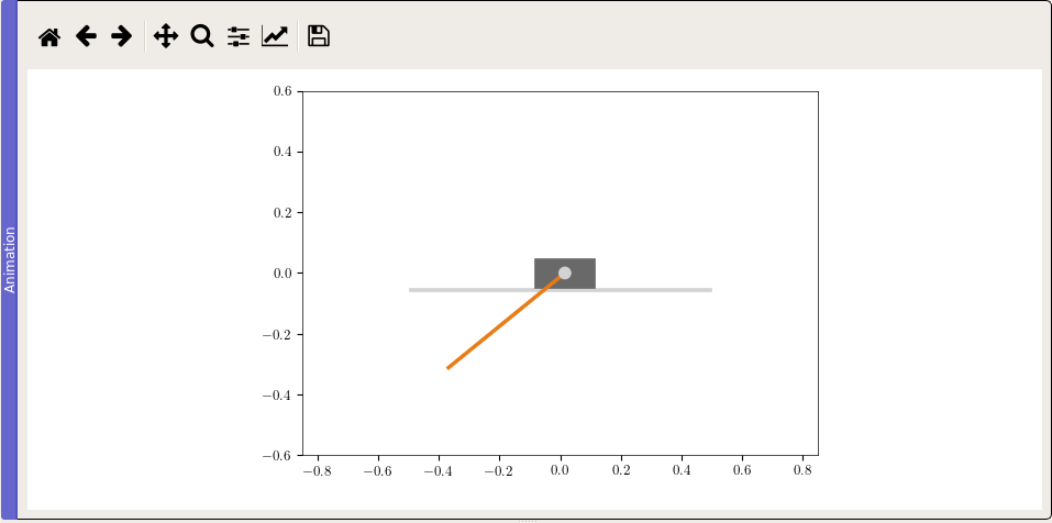
Fig. 9 Matplotlib visualization of the simple pendulum system
If you are looking for a fancier animation, check out the VTK Tutorial.