Closing the Control Loop
Firstly, start PyMoskito from the commandline and reapply the previous steps:
select
PendulumModelasModelchange the initial state of
PendulumModelto[0, 100, 0, 0]select
ODEIntasSolverchange the end time of
Solverto 10select
AdditiveMixerasModelMixer
Now, it gets interesting, select:
the new
BasicControllerasControllerchange
Input AofModelMixertoControllerandselect
SetpointasTrajectory
to generate desired values for out new setup. The setpoint 0 demands that
the cart position (the output defined by our model) should be kept at zero.
To enter string values, type 'Controller' or "Controller"
and remember to press enter to confirm the input.
The Properties window should now look like Fig. 7
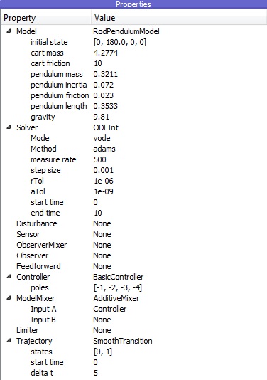
Fig. 7 The properties window with changes for testing applied
Now, hit F5 to run the simulation.
After simulating, you find a few more diagrams in the data section.
Fig. 8 shows the example of the control error.
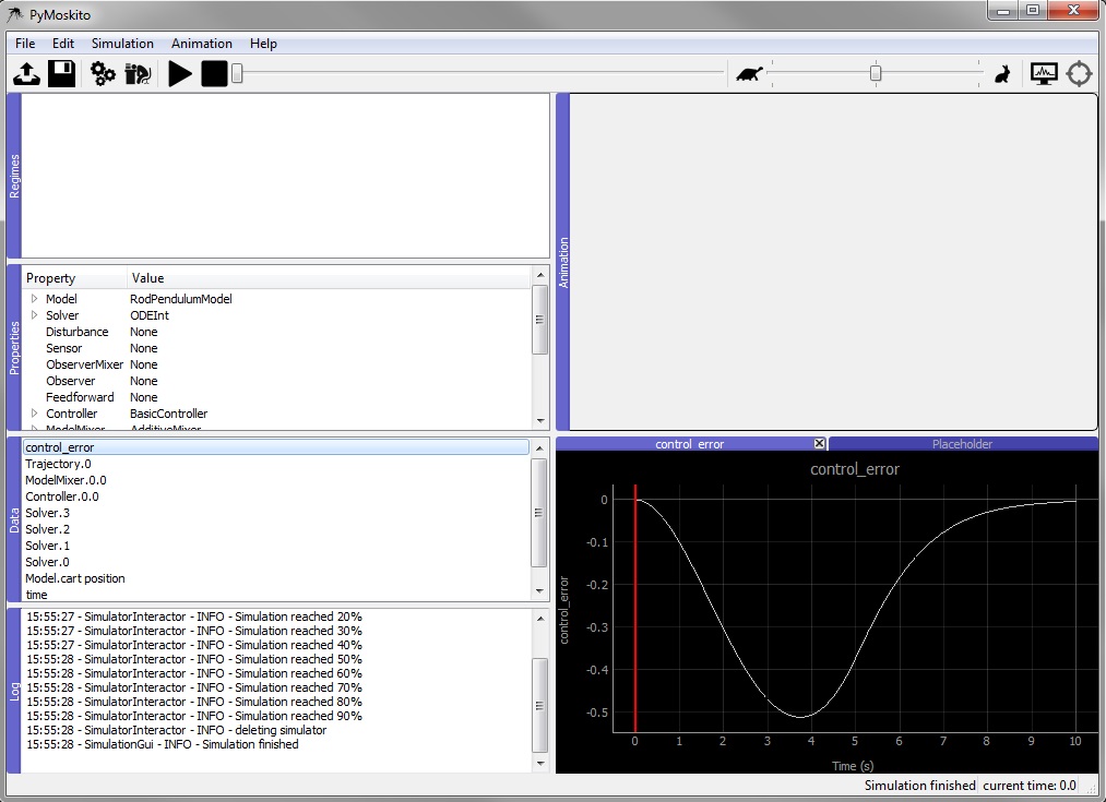
Fig. 8 PyMoskito’s interface with the control error diagram displayed
Feel free to experiment with the settings and see, if the control loop reacts the way you would have predicted. Keep in mind that the implemented controller is static. The control law does not adapt to changes of the model parameters, since the controller gain is calculated from values stored in the controller class. You can use this effect to simulate the situation, where the controller design was based on model parameters that differ from the real parameters of the process.
These were all the fundamental functions of PyMoskito considered necessary to work with it. One more important, but also more advanced feature is the system’s visualization in 2D or 3D. This animation appears in the window at the top right, which remained grey during this tutorial (see Fig. 4, Fig. 6, Fig. 8). For more information on this topic, see the lesson on visualization.